Building Synthetic Data from our Network

Here we load in our Bayesian Network that we built in build_bayesian_network.Rmd. Then we use convenience functions to transform categorical data to continuous where possible.

num_patients <- 1000
snpNames <- c("rs10757278", "rs1333049", "rs4665058", "rs8055236")


library(cvdRiskData)
library(DT)
library(tidyverse)

## Loading tidyverse: ggplot2
## Loading tidyverse: tibble
## Loading tidyverse: tidyr
## Loading tidyverse: readr
## Loading tidyverse: purrr
## Loading tidyverse: dplyr

## Conflicts with tidy packages ----------------------------------------------

## filter(): dplyr, stats
## lag():    dplyr, stats

library(gRain)

## Loading required package: gRbase

## load Bayesian Network
data(cvd_bayes_net)

##build test cases as categorical data
testData <- simulate(cvd_bayes_net, nsim = num_patients)

#transform data into continuous covariates and calculate CVD risk given variables
out <- cvdRiskData:::transformDataSet(testData)

#generate patient IDs
out <- cvdRiskData:::generatePatientIDs(out)

#genotype 0001 modifies the out probability by 4x
out[out$genotype=="0001","outProb"] <- out[out$genotype=="0001","outProb"] * 4

#plot risk score and facet on genotype
out %>% select(outProb, genotype) %>% ggplot(aes(x=outProb)) + geom_histogram() + facet_grid(facets="genotype ~.")

## `stat_bin()` using `bins = 30`. Pick better value with `binwidth`.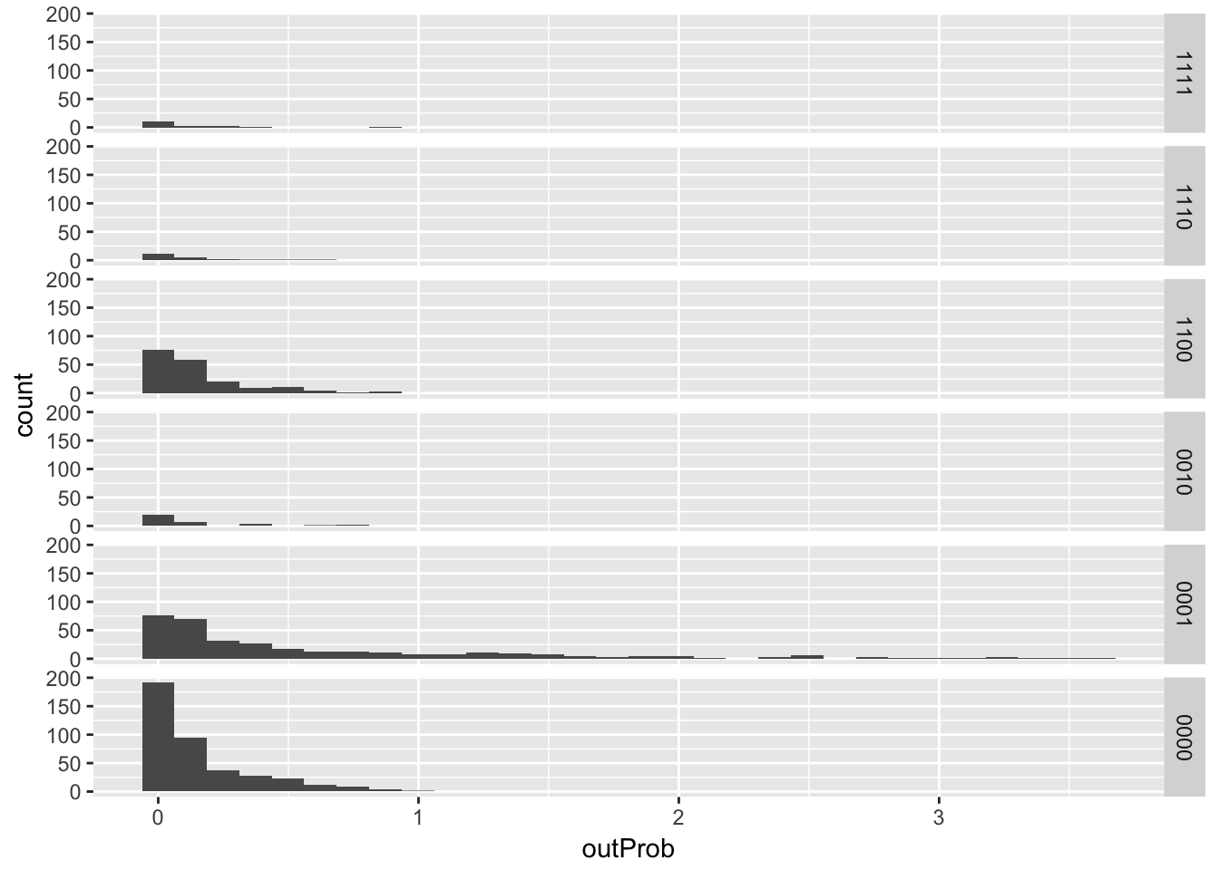

#roll the dice and calculate whether patients have CVD or not given risk
out2 <- cvdRiskData:::callCVD(out) 

#we need to remove 40% of CVD cases to get the right prevalence
cvdInds <- which(out2$cvd == "Y")
toRemove <- floor(length(cvdInds) * 0.6)
indRemove <- sample(cvdInds, toRemove)

out2 <- out2[-indRemove,]
table(out2$cvd)

## 
##   N   Y 
## 765  94

##build genotyping set
gData <- out2 %>% filter(numAge < 45 & numAge >18)  

table(gData$cvd)

## 
##   N   Y 
## 366   8

#make dataset smaller
gDataSmall <- gData[sample(1:nrow(gData), floor(nrow(gData)/3)),]

##bring up snpLookup Table
data("snpLookup")

#build matrix of genotypes
genotypes <- lapply(as.character(gDataSmall$genotype), function(x){snpLookup[[x]]})

outMatrix <- matrix(ncol=4, nrow=length(genotypes), data="D")
colnames(outMatrix) <- snpNames

for(i in 1:length(genotypes)){
  #print(i)
  outMatrix[i,] <- genotypes[[i]]
}

genoFrame <- data.frame(outMatrix)
colnames(genoFrame) <- snpNames

genoData <- data.frame(gDataSmall, genoFrame) 

newData <- out2 %>% select(patientID, age, htn, treat, smoking, race, t2d, gender, numAge, bmi=numBMI, tchol=numTchol, sbp=numHtn,cvd)

genoDataOut <- genoData %>% select(patientID, age, htn, treat, smoking, race, t2d, gender, numAge, bmi=numBMI, tchol=numTchol, sbp=numHtn, rs10757278, rs1333049, rs4665058,  rs8055236, cvd)

#make test and train sets for workshop
inds <- sample(1:nrow(genoDataOut), floor(.85 * nrow(genoDataOut)))
genoDataTrain <- genoDataOut[inds,]
genoDataTest <- genoDataOut[-inds,]

inds <- sample(1:nrow(newData), floor(.85 * nrow(newData)))
newDataTrain <- newData[inds,]
newDataTest <- newData[-inds,]

Here is the data without the genetic covariates (859 patients).

datatable(newData)

Here is the data with genetic covariates (124 patients).

datatable(genoDataOut)

Finally, we save all versions of the data.

write.csv(newData, "../data/fullPatientData.csv", row.names = FALSE)
write.csv(newDataTrain, "../data/fullDataTrainSet.csv", row.names=FALSE)
write.csv(newDataTest, "../data/fullDataTestSet.csv", row.names=FALSE)
write.csv(genoDataTrain, "../data/genoDataTrainSet.csv", row.names=FALSE)
write.csv(genoDataOut, "../data/genoData.csv")
write.csv(genoDataTest, "../data/genoDataTestSet.csv", row.names=FALSE)

save.image("syntheticdata.RData")